Gravitational wave data analysis is mainly done using the coding software Python and therefore there are many Python libraries available that help with the finding of signals within data. This will be a general look at data analysis techniques and no prior knowledge of Python or programming is required.
We’ll look at the data for GW170814, the first gravitational wave detected by both LIGO and Virgo.
Pre-analysis
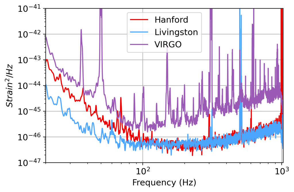
The raw data from the detectors is the form of a timeseries meaning the data is measured across time, but to do any analysis, we need to be able to see the data across frequencies. To do this we generate a power-spectral-density (or PSD), by converting with a Fourier transform (this converts a signal into the frequencies that make it up).
Now the data needs conditioning and the first step is whitening the data. This is because more data is taken for the lower frequencies and therefore any analysis will be biased towards the low end. Whitening allows the data to be spread evenly over the range of frequencies. Then the highest and lowest frequencies we want to look at are set, this is called band passing.
Matched Filtering
Now the data has been conditioned, we can move onto the actual analysis. This is done in the form of matched filtering. Matched filtering is the process of generating a template signal based on guesses about the nature of the signal. Essentially, we guess characteristics about the objects that created the signal (masses, orbit radius, distance from us etc.) and imagine what a gravitational wave that had those parameters would look like, this is our template. Then, we send this template through the data, looking for anything that resembles out template, flagging this as a possible signal.
LIGO sends millions of these templates through their data, each with slightly different parameters and this should locate any signals within the noise.
 Our template waveform


Some Problems
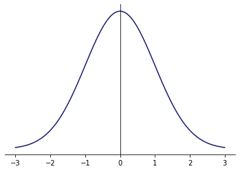
Unfortunately, there are some problems with this technique, mainly to do with the assumptions we tell the computer to make before it sends the template through the data. The two main ones are that the noise follows a Gaussian distribution and that the signal is well-modelled.
A Gaussian distribution is a distribution of probability, meaning that there is more data closer to the average than far away from it. Fundamentally, we are assuming that the noise follows a set pattern, one that we can model very well, as this makes it much easier for the computer to spot signals.
The template we create is based on what we expect a gravitational wave to look like, and quite obviously this means we could be potentially missing many signals as they do not conform to our idea of a gravitational wave. This problem will be solved through research, as we try new models and hopefully find new signals.
Re-Weighting
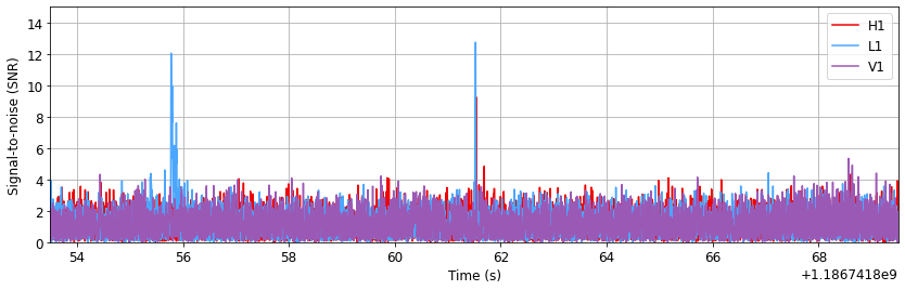
At this point, we have a graph that looks like this:
Looks like we have a total of 2 signals right? Well, to double-check that these are actually signals and not glitches, we can re-weight the data, removing any data points that don’t follow the pattern of Gaussian noise or Gaussian noise plus our template.
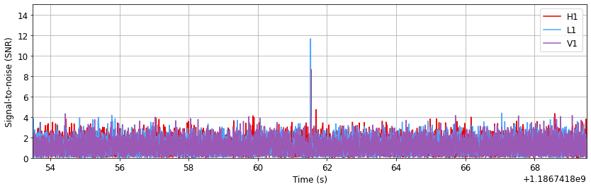
We re-plot the data and get this. What happened to the other signal? Turns out it wasn’t one and was instead likely to be a glitch, learn more about noise and glitches here.
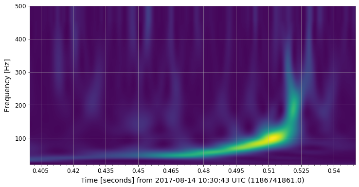
Q-Transform
Now we’ve found our signal, we can graph it using a Q-transform to get a better look at it.
This looks a lot more like the typical signal shape, we can now be pretty happy we’ve found our signal. Now we want to estimate the actual parameters, and we can do this using a Python package called Bilby.
Bilby
Bilby’s main purpose is parameter estimation. This means we can feed it the location of our signal, and some estimations of the nature of the objects that create it and Bilby will do all the work for us, giving us some good approximations to work with. An example plot of the estimations for the two masses and their ratio are shown below. In practice, many more parameters are estimated at once, but this was done for simplicity and to save computing power.
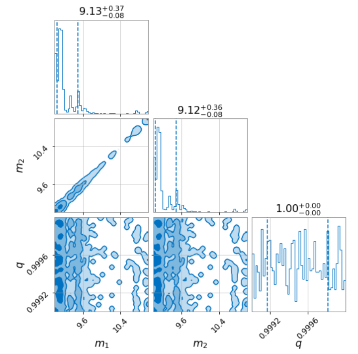
These graphs show the relationship between variables. For example, as the estimate of first mass increases, so does the second (middle left plot above).
We’ve found the signal, visualized it and even got a good estimate for the masses of the objects that made it, our work here is done… for now.
Data: GWOSC